14 区域数据分析

14.1 苏格兰唇癌数据分析

Everything is related to everything else, but near things are more related than distant things.

— Waldo Tobler (Tobler 1970)

空间区域数据分析

空间区域数据的贝叶斯建模

Exact sparse CAR models in Stan 网页文档
Spatial Models in Stan: Intrinsic Auto-Regressive Models for Areal Data 网页文档原始数据和代码，接上面苏格兰唇癌数据分析，用 CmdStanR 更新后的代码
Spatial modeling of areal data. Lip cancer in Scotland INLA 建模

记录 1975-1986 年苏格兰 56 个地区的唇癌病例数，这是一个按地区汇总的数据。

library(sf)
scotlips <- st_read('data/scotland/scotland.shp', crs = st_crs("EPSG:27700"))

Reading layer `scotland' from data source 
  `/home/runner/work/masr/masr/data/scotland/scotland.shp' using driver `ESRI Shapefile'
Simple feature collection with 56 features and 9 fields
Geometry type: MULTIPOLYGON
Dimension:     XY
Bounding box:  xmin: 7150.759 ymin: 529557.2 xmax: 468393.4 ymax: 1218479
Projected CRS: OSGB36 / British National Grid

scotlips

Simple feature collection with 56 features and 9 fields
Geometry type: MULTIPOLYGON
Dimension:     XY
Bounding box:  xmin: 7150.759 ymin: 529557.2 xmax: 468393.4 ymax: 1218479
Projected CRS: OSGB36 / British National Grid
First 10 features:
   SP_ID         NAME ID District Observed Expected pcaff Latitude Longitude
1     12   Sutherland 12       12        5      1.8    16    58.06      4.64
2     13        Nairn 13       13        3      1.1    10    57.47      3.98
3     19    Inverness 19       19        9      5.5     7    57.24      4.73
4     02 Banff-Buchan  2        2       39      8.7    16    57.56      2.36
5     17     Bedenoch 17       17        2      1.1    10    57.06      4.09
6     16   Kincardine 16       16        9      4.6    16    57.00      3.00
7     21        Angus 21       21       16     10.5     7    56.75      2.98
8     50       Dundee 50       50        6     19.6     1    56.45      3.20
9     15      NE Fife 15       15       17      7.8     7    56.30      3.10
10    25    Kirkcaldy 25       25       19     15.5     1    56.20      3.30
                         geometry
1  MULTIPOLYGON (((254301.9 96...
2  MULTIPOLYGON (((292629.6 85...
3  MULTIPOLYGON (((214097.9 84...
4  MULTIPOLYGON (((351078.2 86...
5  MULTIPOLYGON (((239274.9 77...
6  MULTIPOLYGON (((395569.4 80...
7  MULTIPOLYGON (((379822.4 76...
8  MULTIPOLYGON (((357538.2 73...
9  MULTIPOLYGON (((324911.9 71...
10 MULTIPOLYGON (((343283.3 70...

Observed 观测到的患唇癌的案例数
Expected 预期患唇癌的案例数
pcaff: 从事农业、渔业和林业的人口比例（单位：百分比）。

library(ggplot2)
ggplot() +
  geom_sf(data = scotlips, aes(fill = Observed)) +
  scale_fill_viridis_c(option = "plasma", na.value = "white") +
  theme_minimal()

14.1.1 CAR 模型

brms 包的函数 car() 构建 CAR 模型，详情见帮助文档 ?car。

缩写	全称	实现
car	conditional auto-regressive	-
icar	intrinsic CAR	brms
iar	intrinsic auto-regressive Morris 等 (2019)	-
escar	exact sparse CAR	brms
esicar	exact sparse intrinsic CAR	brms
bym2	Besag York Mollié 2 Morris 等 (2019)	brms

# 构造邻接矩阵
library(spdep)
# 根据距离确定近邻关系
scot_nb <- spdep::poly2nb(scotlips, row.names = scotlips$SP_ID)
# 创建邻接矩阵 W
W <- nb2mat(neighbours = scot_nb, style = "B", zero.policy = TRUE)

library(brms)
# 数据变换
scotlips$pcaff2 <- 0.1 * scotlips$pcaff
# 拟合模型
scot_fit_icar <- brm(
  Observed ~ offset(log(Expected)) + pcaff2 + car(W, gr = SP_ID, type = "icar"),
  data = scotlips, data2 = list(W = W), family = poisson(link = "log"),
  refresh = 0, seed = 20232023
)
# 输出结果
summary(scot_fit_icar)

 Family: poisson 
  Links: mu = log 
Formula: Observed ~ offset(log(Expected)) + pcaff2 + car(W, gr = SP_ID, type = "icar") 
   Data: scotlips (Number of observations: 56) 
  Draws: 4 chains, each with iter = 2000; warmup = 1000; thin = 1;
         total post-warmup draws = 4000

Correlation Structures:
      Estimate Est.Error l-95% CI u-95% CI Rhat Bulk_ESS Tail_ESS
sdcar     0.78      0.13     0.56     1.06 1.00      899     1487

Regression Coefficients:
          Estimate Est.Error l-95% CI u-95% CI Rhat Bulk_ESS Tail_ESS
Intercept    -0.19      0.13    -0.44     0.05 1.00     2089     2844
pcaff2        0.32      0.13     0.05     0.57 1.00     1801     2449

Draws were sampled using sampling(NUTS). For each parameter, Bulk_ESS
and Tail_ESS are effective sample size measures, and Rhat is the potential
scale reduction factor on split chains (at convergence, Rhat = 1).

后验线性预测

scotlips$RR <- colMeans(posterior_linpred(scot_fit_icar))
# 相对风险的对数
summary(scotlips$RR)

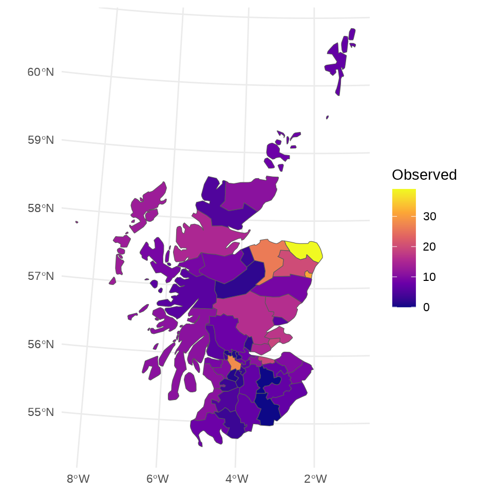
   Min. 1st Qu.  Median    Mean 3rd Qu.    Max. 
 0.3835  1.4173  1.8828  1.9337  2.4005  3.6208

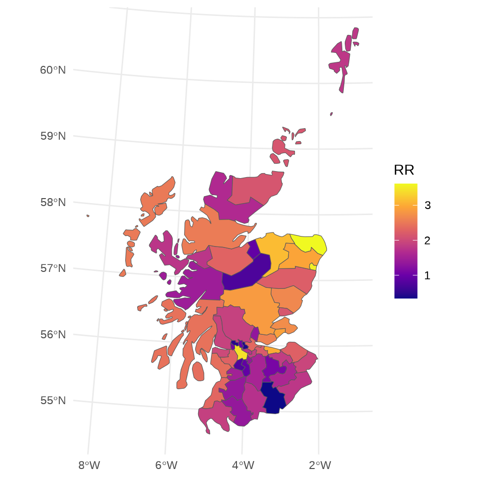
模型的 LOO 值

loo(scot_fit_icar)

Warning: Found 21 observations with a pareto_k > 0.7 in model 'scot_fit_icar'.
We recommend to set 'moment_match = TRUE' in order to perform moment matching
for problematic observations.


Computed from 4000 by 56 log-likelihood matrix.

         Estimate   SE
elpd_loo   -152.8  5.5
p_loo        26.2  2.4
looic       305.6 11.1
------
MCSE of elpd_loo is NA.
MCSE and ESS estimates assume MCMC draws (r_eff in [0.5, 1.4]).

Pareto k diagnostic values:
                         Count Pct.    Min. ESS
(-Inf, 0.7]   (good)     35    62.5%   184     
   (0.7, 1]   (bad)      19    33.9%   <NA>    
   (1, Inf)   (very bad)  2     3.6%   <NA>    
See help('pareto-k-diagnostic') for details.

后验线性预测的拟合值

ggplot() +
  geom_sf(data = scotlips, aes(fill = RR)) +
  scale_fill_viridis_c(option = "plasma", na.value = "white") +
  theme_minimal()

14.1.2 BYM2 模型

响应变量服从泊松分布

BYM-INLA (Blangiardo 等 2013; Moraga 2020)
BYM-Stan (Morris 等 2019; Donegan 2022; Cabral, Bolin, 和 Rue 2022)

将 ICAR 模型更新为 BYM2 模型

# 拟合模型
scot_fit_bym2 <- brm(
  Observed ~ offset(log(Expected)) + pcaff2 + car(W, gr = SP_ID, type = "bym2"),
  data = scotlips, data2 = list(W = W), family = poisson(link = "log"),
  refresh = 0, seed = 20232023
)
# 输出结果
summary(scot_fit_bym2)

 Family: poisson 
  Links: mu = log 
Formula: Observed ~ offset(log(Expected)) + pcaff2 + car(W, gr = SP_ID, type = "bym2") 
   Data: scotlips (Number of observations: 56) 
  Draws: 4 chains, each with iter = 2000; warmup = 1000; thin = 1;
         total post-warmup draws = 4000

Correlation Structures:
       Estimate Est.Error l-95% CI u-95% CI Rhat Bulk_ESS Tail_ESS
rhocar     0.81      0.16     0.41     0.99 1.00      773     1299
sdcar      0.52      0.08     0.38     0.69 1.00     1115     2139

Regression Coefficients:
          Estimate Est.Error l-95% CI u-95% CI Rhat Bulk_ESS Tail_ESS
Intercept    -0.22      0.13    -0.48     0.04 1.00     1949     2559
pcaff2        0.37      0.14     0.08     0.63 1.00     1766     2897

Draws were sampled using sampling(NUTS). For each parameter, Bulk_ESS
and Tail_ESS are effective sample size measures, and Rhat is the potential
scale reduction factor on split chains (at convergence, Rhat = 1).

rhocar 表示 CAR 先验中的参数 \(\rho\)

sdcar 表示 CAR 先验中的参数 \(\sigma\)

loo(scot_fit_bym2)

Warning: Found 20 observations with a pareto_k > 0.7 in model 'scot_fit_bym2'.
We recommend to set 'moment_match = TRUE' in order to perform moment matching
for problematic observations.


Computed from 4000 by 56 log-likelihood matrix.

         Estimate   SE
elpd_loo   -152.6  5.3
p_loo        26.4  2.4
looic       305.2 10.6
------
MCSE of elpd_loo is NA.
MCSE and ESS estimates assume MCMC draws (r_eff in [0.4, 1.6]).

Pareto k diagnostic values:
                         Count Pct.    Min. ESS
(-Inf, 0.7]   (good)     36    64.3%   234     
   (0.7, 1]   (bad)      20    35.7%   <NA>    
   (1, Inf)   (very bad)  0     0.0%   <NA>    
See help('pareto-k-diagnostic') for details.

预测值

scotlips$RR <- colMeans(posterior_linpred(scot_fit_bym2))
# 相对风险的对数
summary(scotlips$RR)

   Min. 1st Qu.  Median    Mean 3rd Qu.    Max. 
 0.3384  1.4162  1.9079  1.9362  2.4052  3.6148

ggplot() +
  geom_sf(data = scotlips, aes(fill = RR)) +
  scale_fill_viridis_c(option = "plasma", na.value = "white") +
  theme_minimal()

14.2 美国各州犯罪率分析

响应变量服从高斯分布的调查数据 (Bivand 2001)

数据集 USArrests 记录 1973 年美国各州每 10 万居民中因谋杀 Murder、袭击 Assault 和强奸 Rape 被警察逮捕的人数以及城市人口所占百分比（可以看作城市化率）。

表格 14.1: 数据集 USArrests（部分）

州名	区域划分	谋杀犯	袭击犯	城市化率	强奸犯
Alabama	South	13.2	236	58	21.2
Alaska	West	10.0	263	48	44.5
Arizona	West	8.1	294	80	31.0
Arkansas	South	8.8	190	50	19.5
California	West	9.0	276	91	40.6
Colorado	West	7.9	204	78	38.7

library(sf)
# 州数据
us_state_sf <- readRDS("data/us-state-map-2010.rds")
# 观测数据
us_state_df <- merge(x = us_state_sf, y = us_arrests,
  by.x = "NAME", by.y = "state_name", all.x = TRUE)

ggplot() +
  geom_sf(
    data = us_state_df, aes(fill = Assault), color = "gray80", lwd = 0.25) +
  scale_fill_viridis_c(option = "plasma", na.value = "white") +
  theme_void()

1973 年美国各州因袭击被逮捕的人数与城市化率的关系：相关分析

代码

library(ggrepel)
ggplot(data = us_arrests, aes(x = UrbanPop, y = Assault)) +
  geom_point(aes(color = state_region)) +
  geom_text_repel(aes(label = state_name), size = 3, seed = 2022) +
  theme_classic() +
  labs(x = "城市化率（%）", y = "因袭击被逮捕人数", color = "区域划分")

阿拉斯加州和夏威夷州与其它州都不相连，属于孤立的情况，下面在空间相关性的分析中排除这两个州。

# 州的中心
centers48 <- subset(
  x = data.frame(x = state.center$x, y = state.center$y),
  subset = !state.name %in% c("Alaska", "Hawaii")
)
# 观测数据
arrests48 <- subset(
  x = USArrests, subset = !rownames(USArrests) %in% c("Alaska", "Hawaii")
)

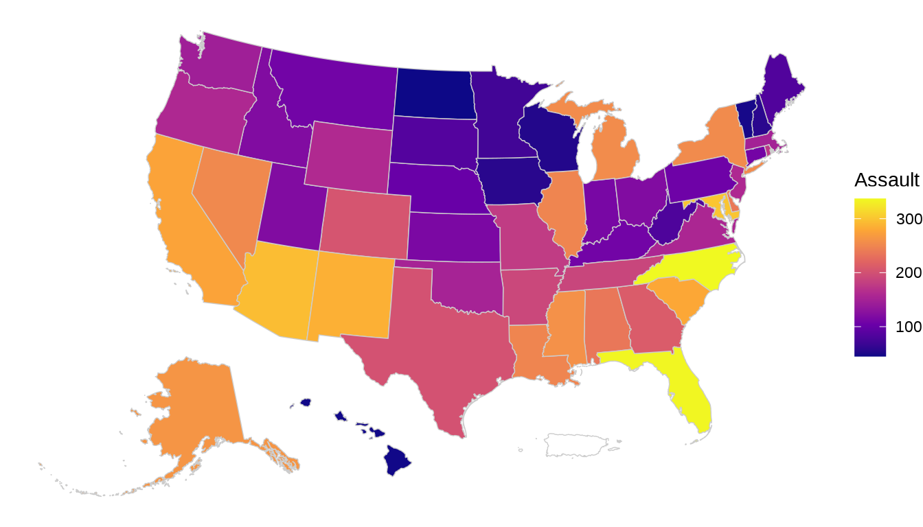
library(spData)
library(spdep)
# KNN K-近邻方法获取邻接矩阵
k4.48 <- knn2nb(knearneigh(as.matrix(centers48), k = 4))
# Moran I test
moran.test(x = arrests48$Assault, listw = nb2listw(k4.48))


    Moran I test under randomisation

data:  arrests48$Assault  
weights: nb2listw(k4.48)    

Moran I statistic standard deviate = 3.4216, p-value = 0.0003113
alternative hypothesis: greater
sample estimates:
Moran I statistic       Expectation          Variance 
      0.294385644      -0.021276596       0.008511253

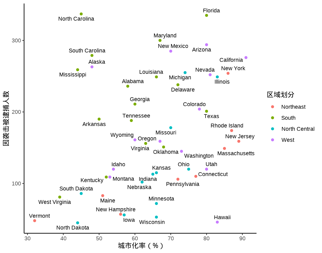
# Permutation test for Moran's I statistic
moran.mc(x = arrests48$Assault, listw = nb2listw(k4.48), nsim = 499)


    Monte-Carlo simulation of Moran I

data:  arrests48$Assault 
weights: nb2listw(k4.48)  
number of simulations + 1: 500 

statistic = 0.29439, observed rank = 498, p-value = 0.004
alternative hypothesis: greater